Chapter 5. Optimizations for Memory Hierarchies

5.1 Introduction

Since the advent of microprocessors, the clock speeds of CPUs have increased at an exponential rate. While the speed at which off-chip memory can be accessed has also increased exponentially, it has not increased at the same rate. A memory hierarchy is used to bridge this gap between the speeds of the CPU and the memory. In a memory hierarchy, the off-chip main memory is at the bottom. Above it, one or more levels of memory reside. Each level is faster than the level below it but stores a smaller amount of data. Sometimes registers are considered to be the topmost level of this hierarchy.

There are two ways in which the intermediate levels of this hierarchy can be organized.

The most popular approach, used in most general-purpose processors, is to use cache memory. A cache contains some frequently accessed subset of the data in the main memory. When the processor wants to access a piece of data, it first checks the topmost level of the hierarchy and goes down until the data sought is found. Most current processors have either two or three levels of caches on top of the main memory. Typically, the hardware controls which subset of state of one level is stored in a higher level. In a cache-based memory hierarchy, the average time to access a data item depends upon the probability of finding the data at each level of the hierarchy. Embedded systems use scratch pad memory in their memory subsystems. Scratch pads are smaller and faster addressable memory spaces. The compiler or the programmer directs where each data item should reside. In this chapter, we restrict our attention to cache-based memory hierarchies. This chapter discusses compiler transformations that reduce the average access latency of accessing data and instructions from memory. The average latency of accesses can be reduced in several ways. The first approach is to reduce the number of cache misses. There are three types of cache misses. Cold misses are the misses that are seen when a data item is accessed for the first time in the program and hence is not found in the cache. Capacity misses are caused when the current working set of the program is greater than the size of the cache. Conflict misses happen when more than one data item maps to the same cache line, thereby evicting some data in the current working set from the cache, but the current working set itself fits within the cache. The second approach is to reduce the average number of cycles needed to service a cache miss. The optimizations discussed later in this chapter reduce the average access latency by reducing the cache misses, by minimizing the access latency on a miss, or by a combination of both. In many processor architectures, the compiler cannot explicitly specify which data items should be placed at each level of the memory hierarchy. Even in architectures that support such directives, the hardware still maintains primary control. In either case, the compiler performs various transformations to reduce the access latency:

1. Code restructuring optimizations: The order in which data items are accessed highly influences which set of data items are available in a given level of cache hierarchy at any given time. In many cases, the compiler can restructure the code to change the order in which data items are accessed without altering the semantics of the program. Optimizations in this category include loop interchange, loop blocking or tiling, loop skewing, loop fusion, and loop fission.
2. Prefetching optimizations: Some architectures do provide support in the instruction set that allows the compiler some explicit control of what data should be in a particular level of the hierarchy. This is typically in the form of prefetch instructions. As the name suggests, a prefetch instruction allows a data item to be brought into the upper levels of the hierarchy before the data is actually used by the program. By suitably inserting such prefetch instructions in the code, the compiler can decrease the average data access latency.
3. Data layout optimizations: All data items in a program have to be mapped to addresses in the virtual address space. The mapping function is often irrelevant to the correctness of the program, as long as two different items are with overlapping lifetimes not mapped to overlapping address ranges. However, this can have an effect on which level of the hierarchy a data item is found and hence on the execution time. Optimizations in this category include structure splitting, structure peeling, and stack, heap, and global data object layout.
4. Code layout optimizations: The compiler has even more freedom in mapping instructions to address ranges. Code layout optimizations use this freedom to ensure that most of the code is found in the topmost level of the instruction cache.

While the compiler can optimize for the memory hierarchies in many ways, it also faces some significant challenges. The first challenge is in analyzing and understanding memory access patterns of applications. While significant progress has been made in developing better memory analyses, there remain many cases where the compiler has little knowledge of the memory behavior of applications. In particular, irregular access patterns such as traversals of linked data structures still thwart memory optimization efforts on the part of modern compilers. Indeed, most of the optimizations for memory performance are designed to handle regular access patterns such as strided array references. The next challenge comes from the fact that many optimizations for memory hierarchies are highly machine dependent. Incorrect assumptions about the underlying memory hierarchy often reduce the benefits of these optimizations and may even degrade the performance. An optimization that targets a cache with a line size of 64 bytes may not be suitable for processors with a cache line size of 128 bytes. Thus, the compiler needs to model the memory hierarchy as accurately as possible. This is a challenge given the complex memory subsystem found in modern processors. In Intel's Itanium, for example, the miss latency of first-level and second-level caches depends upon on factors such as the occupancy of the queue that contains the requests to the second-level cache. Despite these difficulties, memory optimizations are worthwhile, given how much memory behavior dictates overall program performance.

The rest of this chapter is organized as follows. Section 5.2 provides some background on the notion of dependence within loops and on locality analysis that is needed to understand some of the optimizations. Sections 5.3, 5.4, and 5.5 discuss some code restructuring optimizations. Section 5.6 deals with data prefetching, and data layout optimizations are discussed in Section 5.7. Optimizations for the instruction cache are covered in Section 5.8. Section 5.9 briefly summarizes the optimizations and discusses some future directions, and Section 5.10 discusses references to various works in this area.

5.2 Background

Code restructuring and data prefetching optimizations typically depend on at least partial regularity in data access patterns. Accesses to arrays within loops are often subscripted by loop indices, resulting in very regular patterns. As a result, most of these techniques operate at the granularity of loops. Hence, we first present some theory on loops that will be used in subsequent sections. A different approach to understanding loop accesses by using the domain of $\mathcal{Z}$-polyhedra to model the loop iteration space is discussed by Rajopadhye et al. [24].

5.2.1 Dependence in Loops

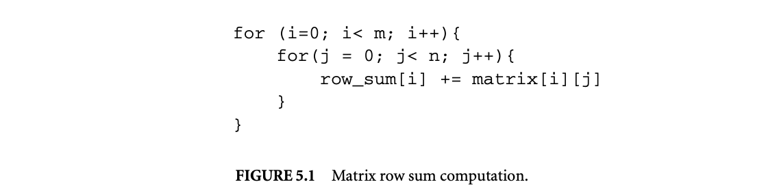
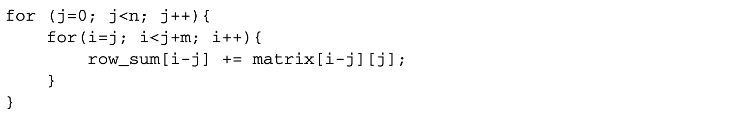
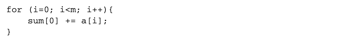
Any compiler transformation has to preserve the semantics of the original code. This is ensured by preserving all true dependences in the original code. Traditional definitions of dependence between instructions are highly imprecise when applied to loops. For example, consider the loop in Figure 5.1 that computes the row sums of a matrix. By the traditional definition of true dependence, the statement row_sum[i]+= matrix[i][j] in the inner loop has a true dependence on itself, but this is an imprecise statement since this is true only for statements within the same inner loop. In other words, row_sum[i+1] does not depend on row_sum[i], and both can be computed in parallel. This shows the need for a more precise definition of dependence within a loop. While a detailed discussion of loop dependence is beyond the scope of this chapter, we briefly discuss loop dependence theory and refer readers to Kennedy and Allen [13].

An important drawback of the traditional definition of dependences when applied to loops is that they do not have any notion of loop iteration. As the above example suggests, if a statement is qualified by its loop iteration, the dependence definitions will be more precise. The following definitions help precisely specify a loop iteration: Normalized iteration number:: If a loop index I has a lower bound of L and a step size of S, then the normalized iteration number of an iteration is given by $\frac{l-k}{S}+1$.

Iteration vector:: An iteration vector of a loop nest is a vector of integers representing loop iterations in which the value of the $k$th component denotes the normalized iteration number of the $k$th outermost loop. As an example, for the loop shown above, the iteration vector i = (1, 2) denotes the second iteration of the j loop within the first iteration of the i loop.

Using iteration vectors, we can define statement instances. A statement instance S(i) denotes the statement S executed on the iteration specified by the iteration vector i. Defining the dependence relations on statement instances, rather than just on the statements, makes the dependence definitions precise. Thus, if S denotes the statement row_sum[i] += matrix[i][j], then there is true dependence between $S(i,j_1)$ and $S(i,j_2)$, where $j_1<j_2<=n$. In general, there can be a dependence between two statement instances $S_1(i_1)$ and $S_2(i_2)$ only if the statement $S_2$ is dependent on $S_1$ and the iteration vector ${\mathbf{i}}_1$ is lexicographically less than or equal to ${\mathbf{i}}_2$. To specify dependence between statement instances, we define two vectors:

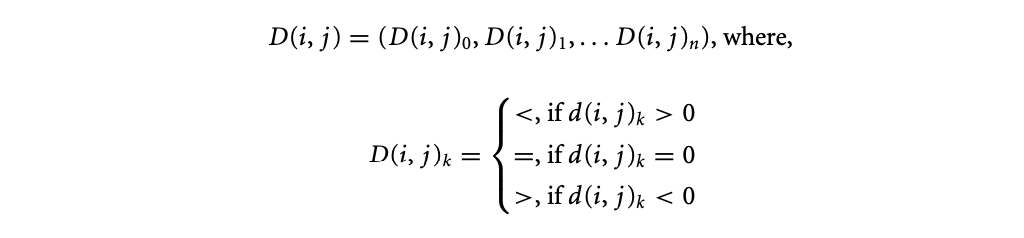
Dependence distance vector:: If there is a dependence from statement $S_i$ in iteration $\mathbf{i}$ to statement $S_j$ in iteration $\mathbf{j}$, then the dependence distance vector $\mathbf{d}(\mathbf{i},\mathbf{j})$ is a vector of integers defined as $\mathbf{d}(\mathbf{i},\mathbf{j})=\mathbf{j}$-$\mathbf{i}$.

Dependence direction vector:: If $\mathbf{d}(\mathbf{i},\mathbf{j})$ is a dependence distance vector, then the corresponding direction vector $\mathbf{D}(\mathbf{i},\mathbf{j})$ is defined as

In any valid dependence, the leftmost non = component of the direction vector must be $<$. The loop transformations described in this chapter are known as reordering transformations. A reordering transformation is one that does not add or remove statements from a loop nest and only reorders the execution of the statements that are already in the loop. Since reordering transformations do not add or remove statements, they do not add or remove any new dependences. A reordering transformation is valid if it preserves all existing dependences in the loop.

5.2.2 Reuse and Locality

Most compiler optimizations for memory hierarchies rely on the fact that programs reuse the same data repeatedly. There are two types of data reuse:

Temporal reuse:: When a program accesses a memory location more than once, it exhibits temporal reuse. Spatial reuse:: When a program accesses multiple memory locations within the same cache line, it exhibits spatial reuse.

These reuses can be due to the same reference or a group of data references. In the former case, the reuse is known as self reuse, and in the latter case, it is known as group reuse. In the loop 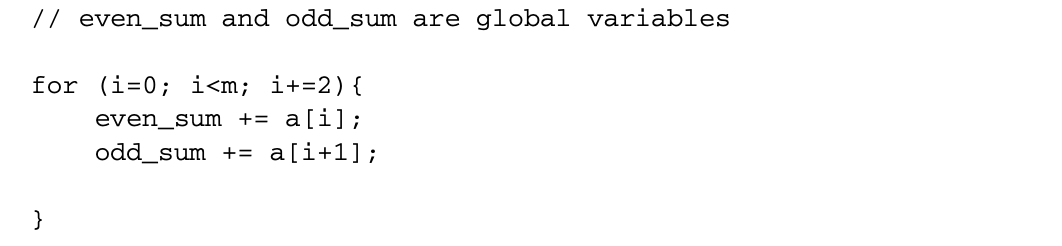even_sum and odd_sum exhibit self-temporal reuse. The references to a[i] and a[i+1] show self-spatial reuse individually and exhibit group-spatial reuse together.

Data reuse is beneficial since a reused data item is likely to be found in the caches and hence incur a low average access latency. If the caches are infinitely large, then all reused data would be found in the cache, but since the cache sizes are finite, a data object D in the cache may be replaced by some other data between two uses of D.

5.2.3 Quantifying Reuse and Locality

The compiler must be able to quantify reuse and locality in order to exploit them. Reuse resulting from array accesses in loops whose subscripts are affine functions of the loop indices can be modeled using linear algebra. Consider an $n$-dimensional array X accessed inside a loop nest $N=(L_1,L_2,\dots L_m)$$m$ loops. Let the loop indices be represented by an $n\times 1$ matrix $i$. Then each access to X can be represented as X[$Ai+C$], where $A$ is an $m\times n$ matrix that applies a linear transformation on $i$, and $C$ is an $m\times 1$ constant vector. For example, an access X[0][i-j] in a loop nest with two loops, whose indices are $\dot{\text{i}}$ and $\dot{\text{j}}$, is represented as X[$Ai+C$], where This access exhibits self-temporal reuse if it accesses the same memory location in two iterations of the loop. If, in iterations $i_1$ and $i_2$, the reference to X accesses the same location, then $A{i}_1+C$ must be equal to $A{i}_2+C$. Let $d=i_1-i_2$. The vector $d$ is known as the reuse distance vector. If a non-null value of $d$ satisfyies the equation $A\times d=0$, then the reference exhibits self-temporal reuse. In other words, if the kernel of the vector space given by $A$ is non-null, then the reference exhibits self-temporal reuse. For the above example, there is a non-null $d$ satisfying the equation since $A\times \left(\genfrac{}{}{0ex}{}{k}{k}\right)=\left(\genfrac{}{}{0ex}{}{0}{0}\right)$. This implies that the location accessed in iteration $(i_1,j_1)$ is also accessed in iteration $(i_1+k,j_1+k)$ for any value of $k$. Group-temporal reuse is identified in a similar manner. If two references $A{i}_1+C_1$ and $A{i}_2+C_2$ to the same array in iterations $i_1$ and $i_2$, respectively, access the same location, then $A{i}_1+C_1$ must be equal to $A{i}_2+C_2$. In other words, if a non-null $d$ satisfies $A\times d=(C_1-C_2)$, the pair of references exhibit group-temporal reuse. If an entry of the $d$ vector is 0, then the corresponding loop carries temporal reuse. The amount of reuse is given by the product of the iteration count of those loops that have a 0 entry in $d$.

An access exhibits self-spatial reuse if two references access different locations that are in the same cache line. We define the term contiguous dimension to mean the dimension of the array along which two adjacent elements of the array are in adjacent locations in memory. In this chapter, all the code examples are in C, where arrays are arranged in row-major order and hence the $n$th dimension of an $n$-dimensional array is the contiguous dimension. For simplicity, it is assumed that two references exhibit self-spatial reuse only if they have the same subscripts in all dimensions except the contiguous dimension. This means the first test for spatial reuse is similar to that of temporal reuse ignoring the contiguous dimension subscript. The second test is to ensure that the subscripts of the last contiguous dimension differ by a value that is less than the cache line size. Given an access $X[Ai+C]$, the entries of the last row of matrix $A$ are coefficients of the affine function used as a subscript in the contiguous dimension. We define a new matrix $A_s$ that is obtained by setting all the columns in the last row of $A$ to 0. If the kernel of $A_s$ is non-null and the subscripts of the contiguous dimension differ by a value less than the cache line size, then the reference exhibits self-spatial reuse. Similarly, group-spatial reuse is present between two references $A{i}_1+C_1$ and $A{i}_2+C_2$ if there is a solution to $A_s\times d=(C_1-C_2)$. Let $i{c}_1,i{c}_2,\dots i{c}_k$ denote the iteration counts of loops that carry temporal reuse in all but the contiguous dimension. Let $s$ be the stride along the contiguous dimension and $cls$ be the cache line size. Then, the total spatial reuse is given by ${\prod }_{i}i{c}_{i_1}\times \frac{d}{s}$.

As described earlier, reuse does not always translate to locality. The term data footprint of a loop invocation refers to the total amount of data accessed by an invocation of the loop. It is difficult to exactly determine the size of data accessed by a set of loops, so it is estimated based on factors such as estimatediteration count. The term localized iteration space[21] refers to the subspace of the iteration space whose data footprint is smaller than the cache size. Reuse translates into locality only if the intersection of the reuse distance vector space with the localized iteration vector space is not empty.

5.3 Loop Interchange

Loop interchange changes the order of loops in a perfect loop nest to improve spatial locality. Consider the loop in Figure 5.2. This loop adds two $m\times n$ matrices. Since multidimensional arrays in C are stored in row-major order, two consecutive accesses to the same array are spaced far apart in memory. If all the three matrices do not completely fit within the cache, every access to a, b, and c will miss in the cache, but a compiler can transform the loop into the following equivalent loop: 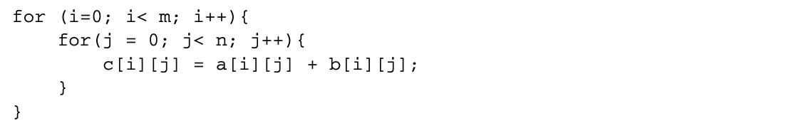The above loop is semantically equivalent to the first loop but results in fewer conflict misses.

As this example illustrates, the order of nesting may be unimportant for correctness and yet may have a significant impact on the performance. The goal of loop interchange is to find a suitable nesting order that reduces memory access latency while retaining the semantics of the original loop. Loop interchange comes under a category of optimizations known as unimodular transformations. A loop transformation is called unimodular if it transforms the dependences in a loop by multiplying it with a matrix, whose determinant has a value of either $-1$ or $1$. Other unimodular transformations include loop reversal, skewing, and so on.

5.3.1 Legality of Loop Interchange

It is legal to apply loop interchange on a loop nest if and only if all dependences in the original loop are preserved after the interchange. Whether an interchange preserves dependence can be determined by looking at the direction vectors of the dependences after interchange. Consider a loop nest $N=(L_1,L_2,\dots L_n)$. Let $\mathbf{D}(\mathbf{i},\mathbf{j})$ be the direction vector of a dependence in this loop nest. If the order of loops in the loop nest is permuted by some transformation, then the direction vector corresponding to the dependence in the permuted loop nest can be obtained by permuting the entries of $\mathbf{D}(\mathbf{i},\mathbf{j})$. To understand this, consider the iteration vectors $i$ and $j$ corresponding to the source and sink of the dependence. A permutation of the loop nest results in a corresponding permutation of the components of $i$ and $j$. This permutes the distance vector $\mathbf{d}(\mathbf{i},\mathbf{j})$ and hence the direction vector $\mathbf{D}(\mathbf{i},\mathbf{j})$. To determine whether $N$ can be permuted to $N^{\prime }=(L_{i_1},L_{i_2},\dots L_{i_n})$, the same permutation is applied to the direction vectors of all dependences, and the resultant direction vectors are checked for validity. As an example, consider the loop

This loop nest has two dependences:

• Dependence from $a[i][j-1]$ to $a[i][j]$, represented by the distance vector $(0,1)$ and the direction vector $(=,<)$
• Dependence from $a[i-1][j+1]$ to $a[i][j]$, represented by the distance vector $(1,-1)$ and the direction vector $(<,>)$

Loop interchange would permute a direction vector by swapping its two components. While the direction vector $(=,<)$ remains valid after this permutation, the vector $(<,>)$ gets transformed to $(>,<)$, which is an invalid direction vector. Hence, the loop nest above cannot be interchanged.

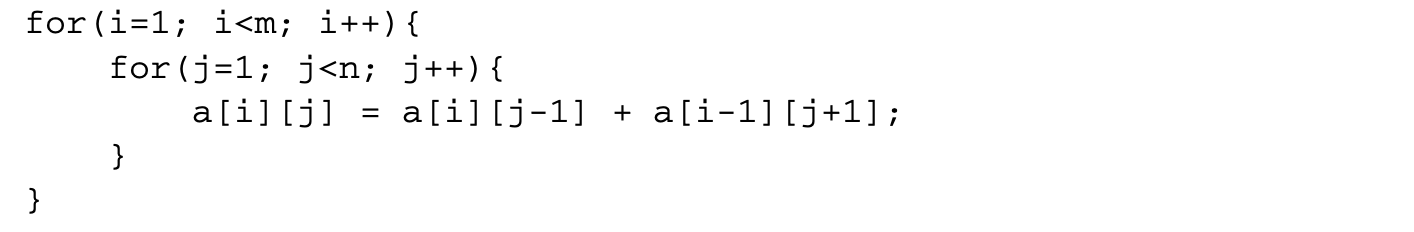
5.3.2 Dependent Loop Indices

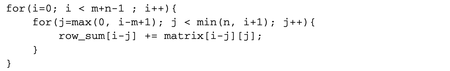
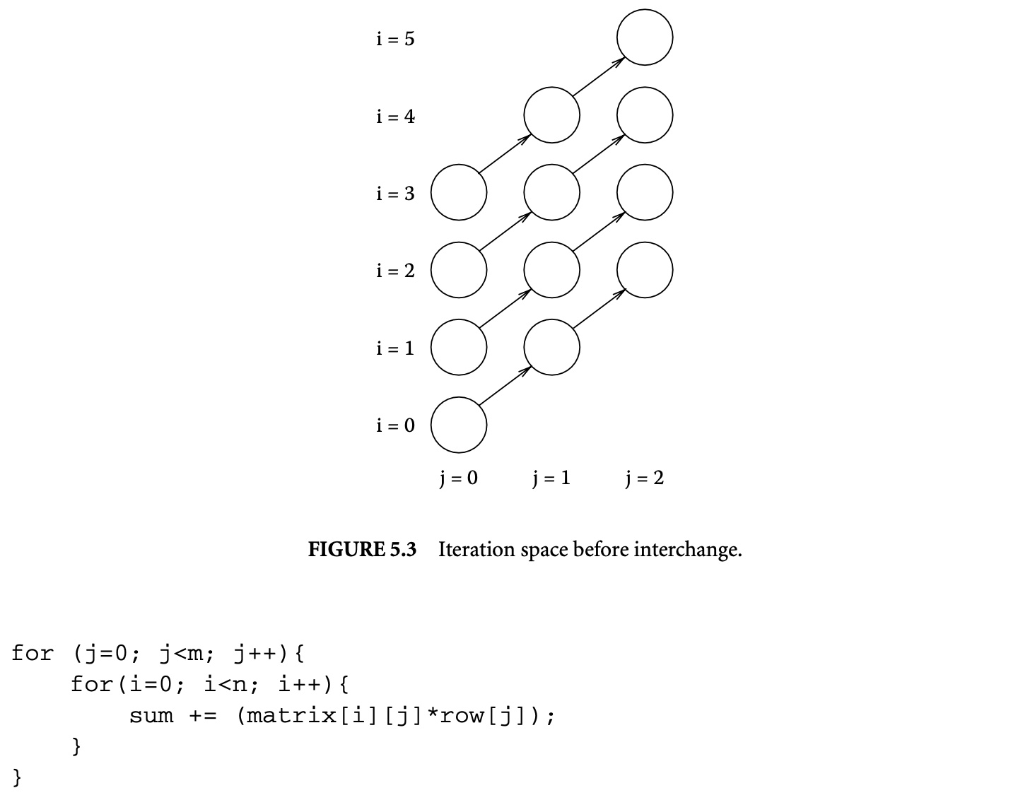
Even if interchange does not violate any dependence, merely swapping the loops may not be possible if the loop indices are dependent on one another. For example, the loop in Figure 5.1 can be rewritten as Except for the change in the bounds of the inner loop index, the loop is semantically identical to the one in Figure 5.1. It has the same dependence vectors, so it must be legal to interchange the loops. However, since the inner loop index is dependent on the outer loop index, the two loops cannot simply be swapped. The indices of the loops need to be adjusted after interchange. This can be done by noting that loop interchange transposes the iteration space of the loop. Figure 5.3 shows the iterations of the original loop for $n=3$ and $m=4$. In Figure 5.4, the iteration space is transposed. This corresponds to the following interchanged loop.

5.3.3 Profitability of Loop Interchange

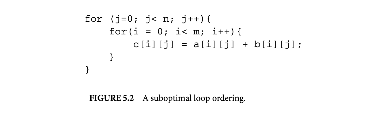
Even if loop interchange can be performed on a loop nest, it is not always profitable to do so. In the example shown in Figure 5.2, it is obvious that traversing the matrices first along the rows and then along the columns is optimal, but when the loop body accesses multiple arrays, each of the accesses may prefer a different loop order. For example, in the following loop

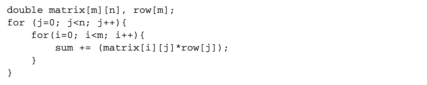
the loop order is suboptimal for accesses to the matrix array. However, this is the best loop order to access the row array. In this loop nest, the element row[j] shows self-temporal reuse between the iterations of the inner loop. Hence, it needs to be accessed just once per iteration of the outer loop. If the loops are interchanged, this array is accessed once per iteration of the inner loop. If the size of the row array is much larger than the size of the cache, then there is no reuse across outer loop iterations.

For this loop nest:

• Number of misses to matrix = $n\times m$
• Number of misses to row = $\frac{n}{ds}$
• Total number of misses = $n\times m+\frac{n}{ds}$

If the loops are interchanged, then

• Number of misses to $\mathtt{matrix}=\frac{n\times m}{ds}$
• Number of misses to $\mathtt{row}=\frac{m\times n}{ds}$
• Total number of misses $=2\times \frac{n\times m}{ds}$

In the above equations, cls denotes the size of the cache line in terms of elements of the two arrays. From this set of equations, it is clear that the interchanged loop is better only when the cache line can hold more than two elements of the two arrays.

5.3.4 A Loop Permutation Algorithm

In theory, one could similarly determine the right order for any given loop nest, but when the maximum depth of a perfect loop nest is $n$, the number of possible loop orderings is $n!$, and computing the total number of misses for those $n!$ loops is prohibitive for a large value of $n$. Instead, we can use some simple set of heuristics to determine an order that is likely to be profitable.

The algorithm in Figure 5.5 computes a good order of loops for the given loop nest $N$. For every loop in $N$, it computes cache_misses(L), which is the estimated number of cache misses when the loop L is made the inner loop. To compute cache_misses(L), the algorithm first computes a set. Each element of this set is either a single array reference or a group of array references that have group reuse. For instance, in the following loop,

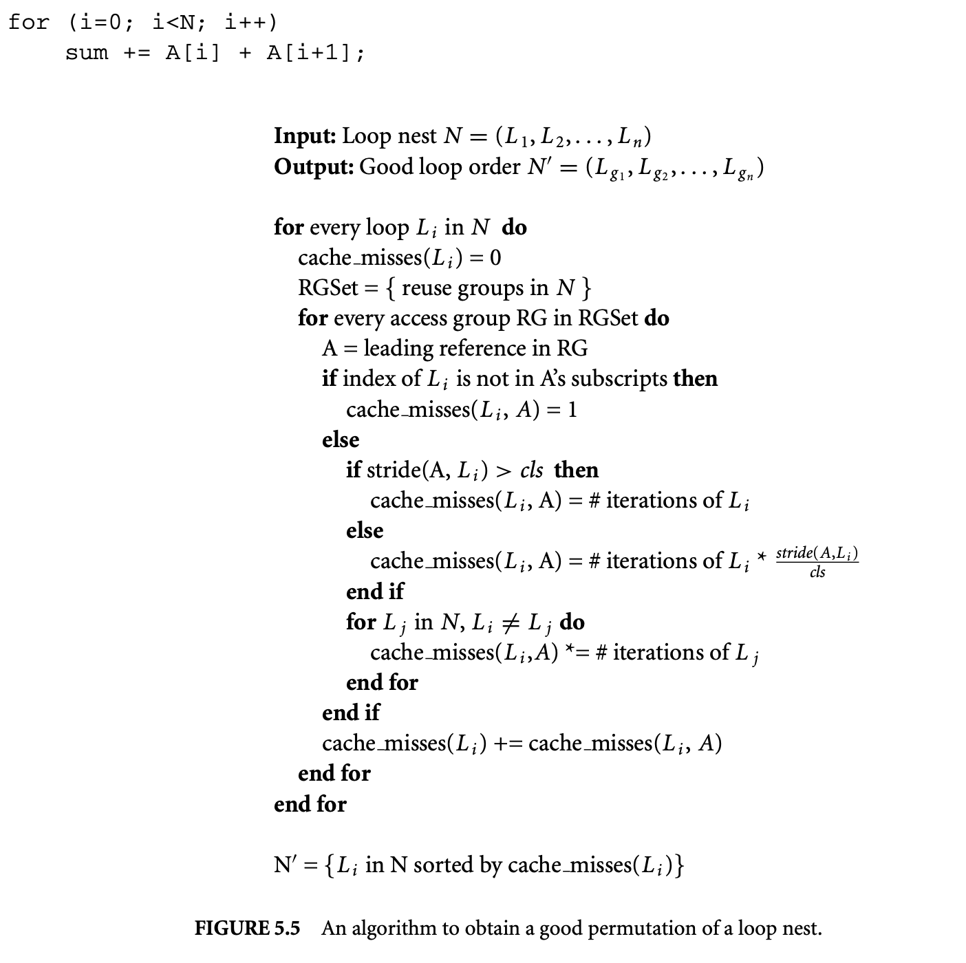
array references $A[i]$ and $A[i+1]$ belong to the same reuse group. Only the leading array reference in a reuse group is used for calculating cache_misses. If a reference does not have $L_i$ in the subscripts, its cost is considered as 1. This is because such a reference will correspond to the same memory location for all iterations of $L_i$ and will therefore miss only once during the first access. If a reference has the index of $L_i$ in one of its subscripts, the stride of the reference is first computed. $stride(A,L_i)$ is defined as the difference in address in accesses of A in two consecutive iterations of $L_i$, where the $i$th component of the iteration vector differs by 1. As an example, $stride(X[i][j],i)$ is 256 in the following code:

If the stride is greater than the cache line size, then every reference to A will miss in the cache, so cache_misses is incremented by the number of iterations of $L_i$. If the stride is less than cache line size, then only one in every $\frac{cls}{stride}$ accesses will miss in the cache. Hence, the number of iterations of $L_i$ is divided by $\frac{cls}{stride}$ and added to cache_misses($L_i$). Then, for each reference, cache_misses($L_i$) is multiplied by the iteration counts of other loops whose indices are used as some subscript of A. Finally, the cache_misses for all references are added together.

After cache_misses($L_i$) for each loop $L_i$ is computed, the loops are sorted by cache_misses in descending order, and this is to obtain a good loop order. In other words, the loop with the lowest estimated cache misses is a good candidate for the innermost loop, the loop with the next lowest cache misses is a good candidate for the next innermost loop, and so on.

To see how this algorithm works, it is applied to the loop Let $L_i$ denote the loop with induction variable i and $L_j$ denote the loop with induction variable j. For the loop nest with i as the induction variable:

1. cache_misses($L_i$, row) = $n$, since $i$ is not a subscript in row.
2. cache_misses($L_i$, matrix) = $m^{\ast }n$. Here we assume that $n$ is a large enough number so that stride($n$, $L_i$) is greater than the cache line size.
3. cache_misses($L_i$) = $n+n^{\ast }m$.

For the loop $L_j$:

1. cache_misses($L_j$, row) = $m^{\ast }{n}^{\ast }$sizeof(double)/cls
2. cache_misses($L_j$, matrix) = $m^{\ast }{n}^{\ast }$sizeof(double)/cls
3. cache_misses($L_j$) = $2^{\ast }{m}^{\ast }{n}^{\ast }$sizeof(double)/cls

If the cache line can hold at least two doubles, cache_misses($L_j$) is less than cache_misses($L_i$), and therefore $L_j$ is the candidate for the inner loop position.

While the algorithm in Figure 5 determines a good loop order in terms of profitability, it is not necessarily a valid order, as some of the original dependences may be violated in the new order. The order produced by the algorithm is therefore used as a guide to obtain a good legal order. This can be done in the following manner:

1. Pick the best candidate for the outermost loop among the loops that are not yet in the best legal order.
2. Assign it to the outermost legal position in the best legal order.
3. Repeat steps 1 and 2 until all loops are assigned a place in the best legal order.

Kennedy and Allen [13] show why the resulting order is always a legal order.

5.4 Loop Blocking

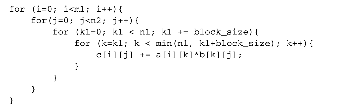
A very common operation in many scientific computations is matrix multiplication. The code shown below is a simple implementation of the basic matrix multiplication algorithm. 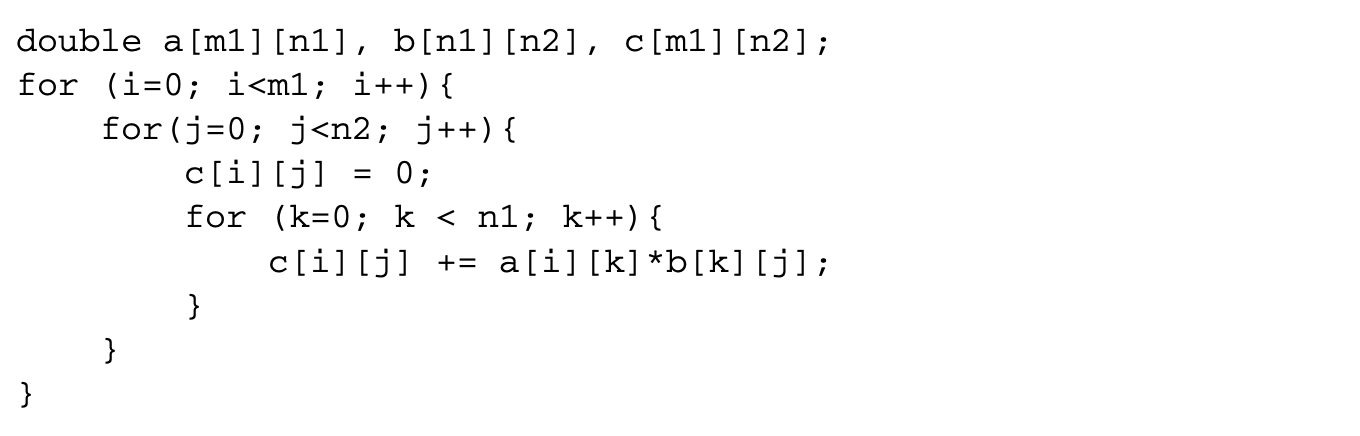This code has a lot of data reuse. For instance, every row of matrix a is used to compute n2 different elements of the product matrix c. However, this reuse does not translate to locality if the matrices do not fit in the cache. If the matrices do not fit in the cache, the loop also suffers from capacity misses that are not eliminated by loop interchange. In this case, the following transformed loop improves locality:

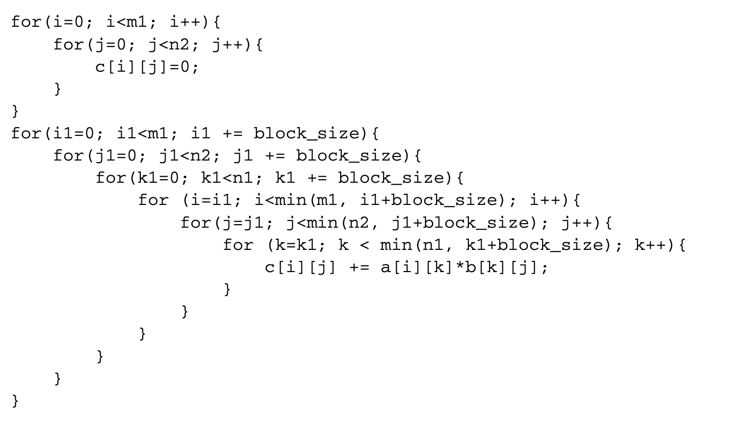
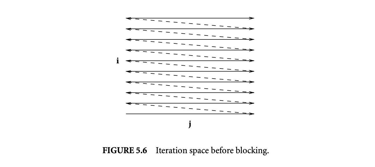
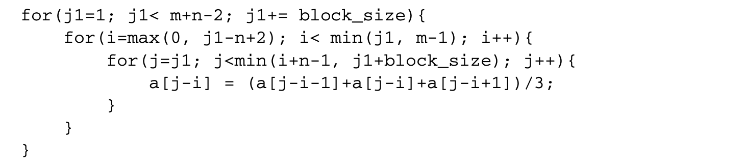
First the initialization of the matrix c is separated out from the rest of the loop. Then, a transformation known as blocking or tiling is applied. If the value of block_size is chosen carefully, the reuse in the innermost three loops translates to locality. Figures 5.6 and 5.7 show the iteration space of a two-dimensional loop nest before and after blocking. In this example, the original iteration space has been covered by using four nonoverlapping rectangular tiles or blocks. In general, the tiles can take the shape of a parallelepiped for an $n$-dimensional iteration space. A detailed discussion of tiling shapes can be found in Rajopadhye [24]. The basic transformation used in blocking is called strip-mine and interchange. Strip mining transforms a loop into two nested loops, with the inner loop iterating over a small strip of the original loop and the outer loop iterating across strips. Strip mining the innermost loop in the matrix multiplication example results in the following loop nest: Assuming block_size is smaller than n1, the innermost loop now executes fewer iterations than before, and there is a new loop with index k1. After strip mining, the loop with index k1 is interchanged with the two outer loops, resulting in blocking along one dimension: 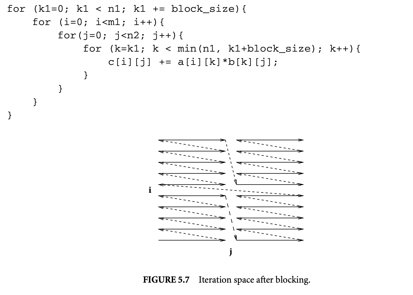Doing strip-mine and interchange on the $\mathtt{i}$ and $\mathtt{j}$ loops also results in the blocked matrix multiplication code shown earlier. An alternative approach to understand blocking in terms of clustering and tiling matrices is discussed by Rajopadhye [24].

5.4.1 Legality of Strip-Mine and Interchange

Let $L_k$ be a loop which is to be strip mined into an outer loop $L_k^{\prime }$ and an inner loop $L_k^{\prime \prime }$. Let $L_j$ be the loop with which the loop $L_k^{\prime \prime }$ is to be interchanged. Strip mining $L_k$ is always a legal transformation since it does not alter any of the existing dependences and only relabels the iteration space of the loop. Thus, the legality of blocking depends on the legality of the interchange of $L_k^{\prime }$ and $L_j$, but determining the legality of this interchange requires strip mining $L_k$, which necessitates the recomputation of the direction vectors of all the dependences. A faster alternative is to test the legality of interchanging $L_j$ with $L_k$ instead. While the legality of this interchange ensures the correctness of blocking, this test is conservative and may prevent valid strip-mine and interchange in some cases ¹.

5.4.2 Profitability of Strip-Mine and Interchange

We now discuss the conditions under which strip-mine and interchange transformation is profitable, given the strip sizes, which determine the block size. For a discussion of optimal block sizes refer to Rajopadhye [24] (Chapter 15 in this text).

Given a loop nest $N=(L_1,L_2\dots L_n)$, a loop $L_k$ and another loop $L_j$, where $L_k$ is nested within $L_j$, the profitability of strip mining $L_k$ and interchanging the by-strip loop with $L_j$ depends on the following:

• The reuse carried by $L_j$
• The data footprint of all inner loops of $L_k$
• The cost of strip mining $L_k$

The goal of strip mining $L_k$ and interchanging the by-strip loop with $L_j$ is to ensure that reuse carried by $L_j$ is translated into locality. For this to happen, $L_j$ must carry reuse between its iterations. This can happen under any of the following circumstances:

• There is some dependence carried by $L_j$. If $L_j$ carries some dependence, it means an iteration of $L_j$ reuses a location accessed by some earlier iteration of $L_j$.
• There is an array index that does not have the index of $L_j$ in any of its subscripts.
• The index of $L_j$ is used as a subscript in the contiguous dimension, resulting in spatial reuse.

The data footprint of $L_j$ must be larger than the cache size, as otherwise the reuse carried by $L_j$ lies within the localized iteration space. The data footprint of $L_k$ must also be larger than the cache size, as otherwise it is sufficient to strip-mine some other loop between $L_j$ and $L_k$. Finally, the benefits of reuse must still outweigh the cost of strip mining $L_k$. Strip mining can cause a performance penalty in two ways:

• If the strips are not aligned to cache line boundaries, it would reduce the spatial locality of array accesses that have the index of $L_k$ as the subscript in the contiguous dimension.
• Every dependence carried by the loop $L_k$ shows decreased temporal locality.

Typically, the cost of doing strip-mine and interchange is small and is often outweighed by the benefits.

5.4.3 Blocking with Skewing

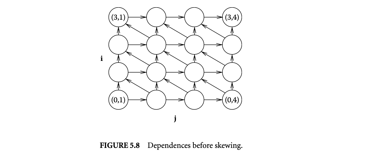
In loop nests where interchange violates dependences, loop skewing can be applied first to enable loop interchange. Consider the loop iteration shown in Figure 5.8. The outer loop of this nest is indexed by $\mathbf{i}$, and the inner loop by $\mathbf{j}$. Even if it is profitable, the diagonal edges from iteration vector $(\mathbf{i},\mathbf{j})$ to $(\mathbf{i}+1,\mathbf{j}-1)$prevent loop interchange, but the same loop can be transformed to the one in Figure 5.9, which allows loop interchange. This transformation is known as loop skewing. Given two loops, the inner loop can be skewed with respect to the outer loop by adding the outer loop index to the inner loop index. Consider a dependence with direction vector $(<,>)$. This pair of loops does not permit loop interchange. Consider two iteration vectors $(i1,j1)$ and $(i2,j2)$, which are the source and target, respectively, of the dependence. Let $(d1,d2)$ be the distance vector corresponding to this dependence, where $(d1,d2)=(i1-i2,j1-j2)$. The goal is to transform this distance vector into $(d1,d2+f\times d1)$, where $f\times d1>=|d2|$, so that the direction vector becomes either $(<,<)$ or $(<,=)$, which permits loop interchange. This can be achieved by multiplying the outer loop index and adding the product to the inner loop index. Thus, the two iteration vectors become $(i1,j1+f.i1)$ and $(i2,j2+f.i2)$, and the distance vector becomes $(i1-i2,j1-j2+f.(i1-i2))$, which is equal to $(d1,d2+f.d1)$.

The loop shown in Figure 5.8 applies an averaging filter $m$ times on an array as shown below: 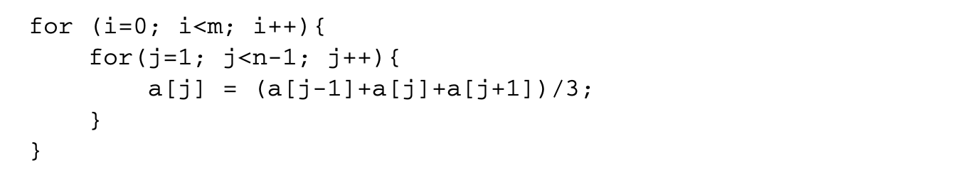The dependences in this loop are characterized by three dependence distance vectors $(0,1),(1,0)$, and $(1,-1)$, which are depicted in Figure 5.8, for the case where $m$ takes a value of 4 and $n$ takes a value of 6. While the $\mathbf{j}$ loop can be strip mined into two loops with induction variables $j1$ and $\mathbf{j}$, the $j1$ loop cannot be interchanged with the $\mathbf{i}$ loop because of the dependence represented by $(-1,1)$. We skew the inner $\mathbf{j}$ loop with respect to the outer $\mathbf{i}$ loop.

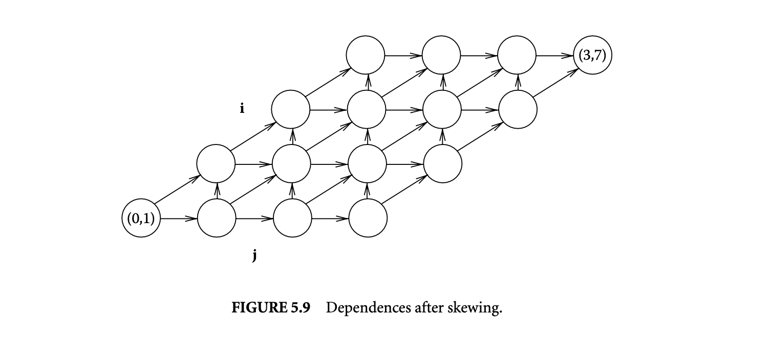
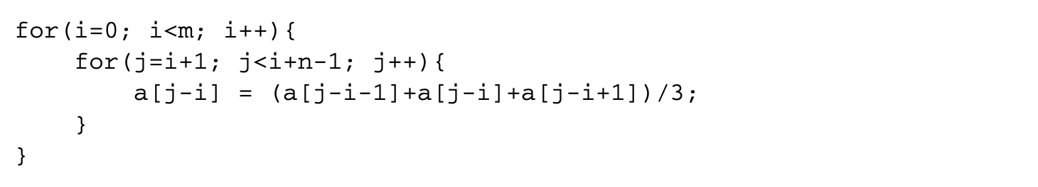
Since a distance vector of $(1,0)$ allows interchange, the value of $f$ is chosen as 1. Figure 5.9 shows the dependences in the loop after applying skewing. This corresponds to the following loop: Strip mining the loop with index j results in the following code: 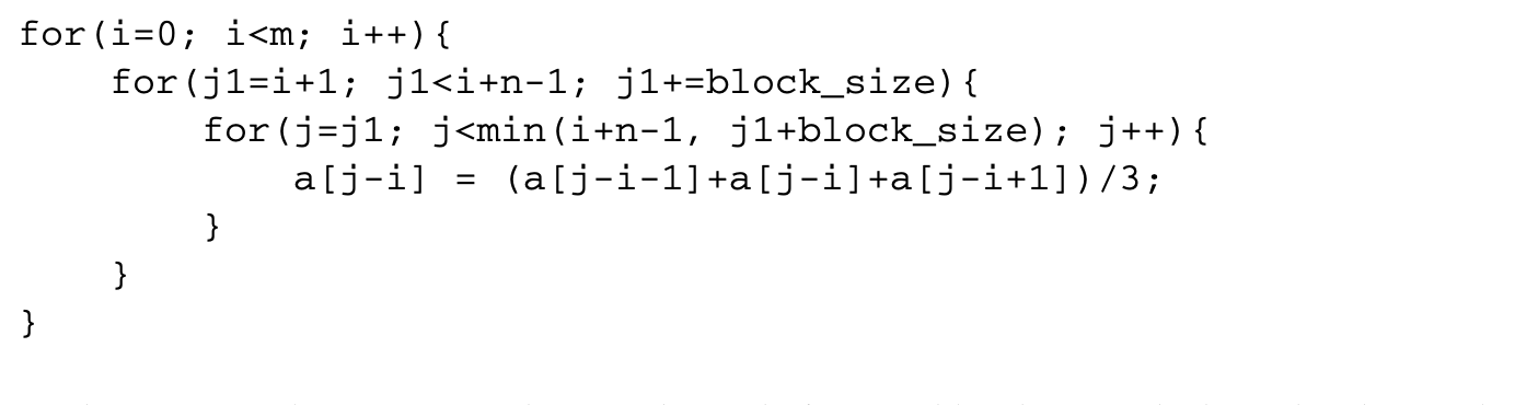The outer two loops can now be interchanged after suitably adjusting the bounds. This results in the tiled loop:

5.5 Other Loop Transformations

5.5.1 Loop Fusion

When there is reuse of data across two independent loops, the loops can be fused together, provided their indices are compatible. For example, the following set of loops: 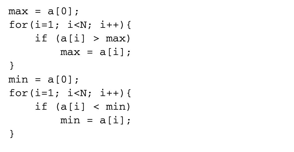can be fused together into a single loop:

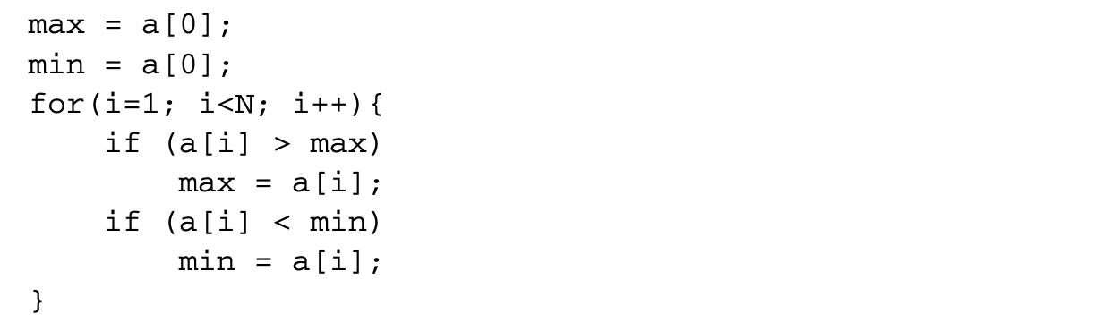
If the value of N is large enough that the array does not fit in the cache, the original loop suffers from conflict misses that are minimized by the fused loop. Loop fusion is often combined with loop alignment. Two loops may have compatible loop indices, but the bounds may be different. For example, if the first loop computes the maximum of all $N$ elements and the second loop computes the minimum of only the first $N/2$ elements, the indices have to be aligned. This is done by first splitting the max loop into two, one iterating over the first $N/2$ elements and the other over the rest of the elements. Then the loop computing the minimum can be fused with the first portion of the loop computing the maximum.

5.5.2 Loop Fission

Loop fission or loop distribution is a transformation that does the opposite of loop fusion by transforming a loop into multiple loops such that the the body of the original loop is distributed across those loops. To determine whether the body can be distributed, the program dependence graph (PDG) of the loop body is constructed first. Different strongly connected components of the PDG can be distributed into different loops, but all nodes in the same strongly connected component have to be in the same loop. For example, the following loop, 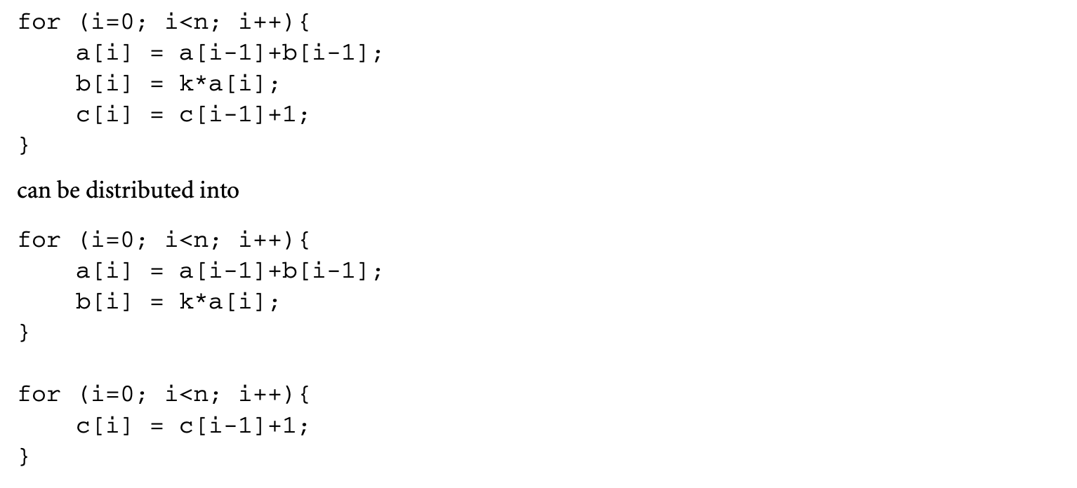since the statement $c[i]=c[i-1]+1$ is independent of the other two statements, which are dependent on each other. Loop fission reduces the memory footprint of the original loop. This is likely to reduce the capacity misses in the original loop.

5.6 Data Prefetching

Data prefetching differs from the other loop optimizations discussed above in some significant aspects:

• Instead of transforming the data access pattern of the original code, prefetching introduces additional code that attempts to bring in the cache lines that are likely to be accessed in the near future.

• Data prefetching can reduce all three types of misses. Even when it is unable to avoid a miss, it can reduce the time to service that miss.

• While the techniques described above are applicable only for arrays, data prefetching is a much more general technique.

• Prefetching requires some form of hardware support.

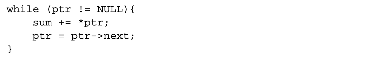
Consider the simple loop

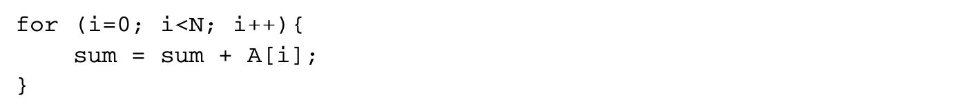
This loop computes the sum of the elements of the array A. The cache misses to the array A are all cold misses. To avoid these misses, prefetching code is inserted in the loop to bring into the cache an element that is required some pd iterations later: 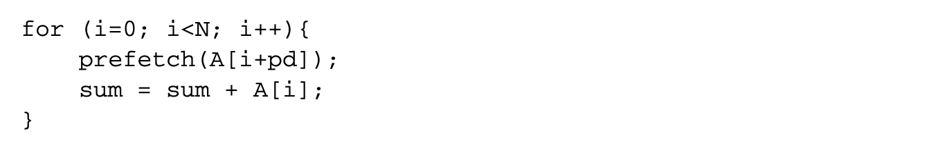The value $pd$ above is referred to as the prefetch distance, which specifies the number of iterations between the prefetching of a data element and its actual access. If the value of $pd$ is carefully chosen, then on most iterations of the loop, the array element that is accessed in that iteration would already be available in the cache, thereby minimizing cold and capacity misses.

5.6.1 Hardware Support

In the above example, we have shown prefetch as a function routine. In practice, prefetch corresponds to some machine instruction. The simplest option is to use the load instruction to do the prefetch. By loading the value to some unused register or a register hardwired to a particular value and making sure the instruction is not removed by dead code elimination, the array element is brought into the cache. While this has the advantage of requiring no additional support in the instruction set architecture (ISA), this approach has some major limitations. First, the load instructions have to be nonblocking. A load instruction is nonblocking if the load miss does not stall other instructions in the pipeline that are independent of the load. If the load blocks the pipeline, the prefetches themselves would suffer cache misses and block the pipeline, defeating the very purpose of prefetching. This is not an issue in most modern general-purpose processors, where load instructions are nonblocking. The second, and major, limitation is that since executing loads can cause exceptions, prefetches might introduce new exceptions in the transformed code that were not there in the original code. For instance, the code example shown earlier might cause an exception when it tries to access an array element beyond the length of the array. This can be avoided by making sure an address is prefetched only if it is guaranteed not to cause an exception, but this would severely limit the applicability of prefetching. To avoid such issues, some processors have special prefetch instructions in their instruction set architecture. These instructions do not block the pipeline and silently ignore any exceptions that are raised during their execution. Moreover, they typically do not use any destination register, thereby improving the register usage in code regions with high register pressure.

5.6.2 Profitability of Prefetching

Introducing data prefetching does not affect the correctness of a program, except for the possibility of spurious exceptions discussed above. When there is suitable ISA support to prevent such exceptions, the compiler has to consider only the profitability aspect when inserting prefetches. For a prefetch instruction to be profitable, it has to satisfy two important criteria: accuracy and timeliness.

Accuracy refers to the fact that a prefetched cache line is actually accessed later by the program. Prefetches may be inaccurate because of the compiler's inability to determine runtime control flow. Consider the following loop: 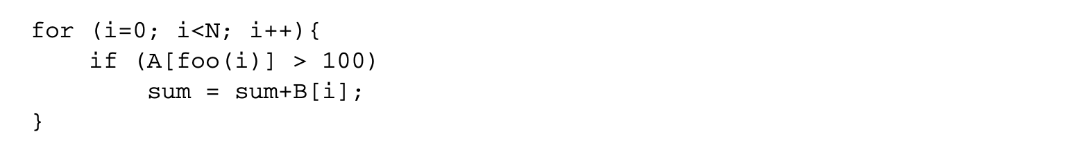A prefetch for the array B inserted at iteration $i$ is accurate only if the element B[i+pd] is accessed later, but this depends on A[foo(i+pd)], and it may not always be safe to compute foo(i+pd). Even if it is safe to do so, the cost of invoking foo may far outweigh the potential benefits of prefetching, forcing the compiler to insert prefetches unconditionally for every future iteration. As will be described later, prefetching of a loop traversing a recursive data structure could also be inaccurate. The accuracy of a prefetch is important because useless prefetches might evict useful data -- data that will definitely be accessed in the future -- from the cache line and increase the memory traffic, thereby degrading the performance.

Accuracy alone does not guarantee that a prefetch is beneficial. If we set the value of $pd$ to be 0, then we can guarantee that the prefetch is accurate by issuing it right before the access, but this obviously does not result in any benefit. A prefetch is timely if it is issued at the right time, so that, when the access happens, it finds the data in the cache. The prefetch distance determines the timeliness of a prefetch for a given loop. Let $h$ be the average schedule height of a loop iteration and $pd$ be the prefetch distance. Then the number of cycles separating the prefetch and the actual access is roughly $pd\ast h$. This value must be greater than the access latency without prefetch for the access to be a hit in the L1 cache. At the same time, if this value is too high, the probability of the prefetched cache line being displaced subsequently, before the actual access, increases, thereby reducing the benefits of the prefetch. Thus, determining the right prefetch distance for a given loop is a crucial step in prefetching implementations.

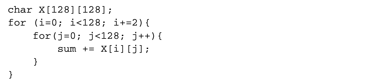
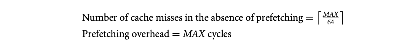
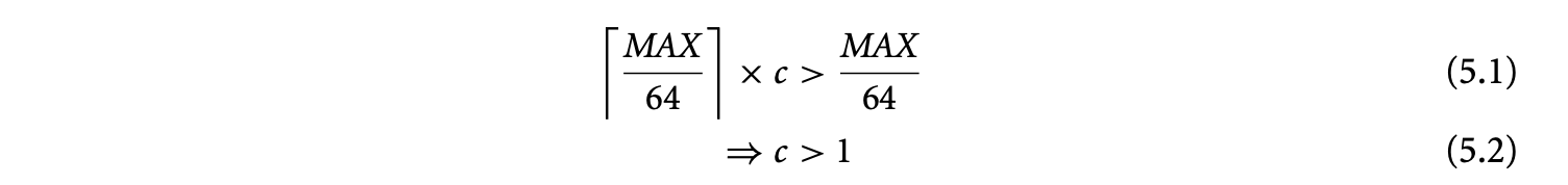
A third factor that determines the benefits of prefetching is the overhead involved in prefetching. The following example shows how the prefetching overhead could negate the benefits of prefetching. Consider the code fragment 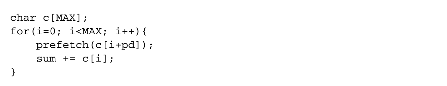This code is the same as the example shown earlier, except that it sums up an array of chars. Assume that this code is executed on a machine with an issue width of 1, and the size of the L1 cache line is 64 bytes. Let $c$ be the number of cycles required to service a cache miss. Under this scenario, Even if all the misses are prefetched,

For prefetching to be beneficial,

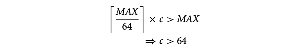
If the miss latency for this access without prefetching is $<$64 cycles, then the overhead of prefetching outweighs its benefits. In such cases, optimizations such as loop splitting or loop unrolling can make prefetching still be profitable. If the value of $MAX$ is determined, either statically or using profiling, to be a large number, unrolling the loop 64 times will make prefetching profitable. After unrolling, only one prefetch is issued per iteration of the unrolled loop, and hence the prefetching overhead reduces to $\frac{MAX}{64}$ cycles. For prefetching to be beneficial in this unrolled loop, Thus, as long as the cost of a cache miss is more than one cycle, prefetching will be beneficial.

5.6.3 Prefetching Affine Array Accesses

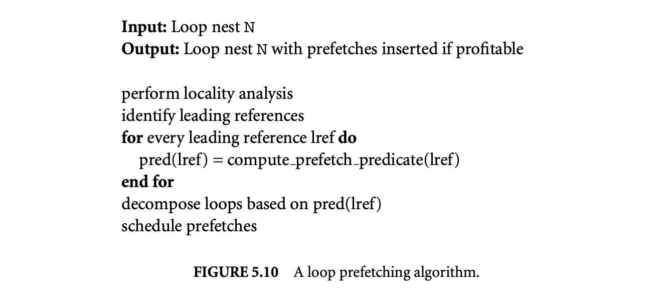
Figure 5.10 outlines an algorithm by Mowry et al. [21] that issues prefetches for array accesses within a loop.

The prefetching algorithm consists of the following steps:

1. Perform locality analysis. The first step of the algorithm is to obtain reuse distance vectors and intersect them with the localized iteration space to determine the locality exhibited by the accesses in the loop.

2. Identify accesses requiring prefetches. All accesses exhibiting self-reuse are candidates for prefetching. When accesses exhibit group reuse, only one of the accesses needs to be prefetched. Among references that exhibit group reuse, the one that is executed first is called the leading reference. It is sufficient to prefetch only the leading reference of each group.

3. Compute prefetch predicates. When a reference has spatial locality, multiple instances of that reference access the same cache line, so only one of them needs to be prefetched. To identify this, every instance of an access is associated with a prefetch predicate. An instance of a reference is prefetched only if the predicate associated with it is 1. Since all references are affine array accesses, the predicates are some functions of the loop indices. As an example, consider the following loop nest: Assuming that the arrays are aligned to cache line boundaries, the prefetch predicate for sum is $(i==0)$ and for a is $\text{(a mod n)==0}$, where n is the number of elements of a in a cache line.

4. Perform loop decomposition. One way to ensure that a prefetch is inserted only when the predicate is true is to use a conditional statement based on the prefetch predicate or, if the architecture supports it, use predicate registers to guard the execution of the prefetch. This requires computing the predicate during every iteration of the loop, which takes some cycles, and issuing the prefetch on every iteration, which takes up issue slots. Since the prefetch predicates are well-defined functions of the loop indices, a better approach is to decompose the loop into sections such that all iterations in a particular section either satisfy the predicate or do not satisfy the predicate. The code above, with respect to the reference to array a, satisfies the predicate in iterations 0, n, 2n, and so on and does not satisfy the predicates in the rest of the iterations. There are many ways to decompose the loops into such sections. If a prefetch is required only during the first iteration of a loop, then the first iteration can be peeled out of the loop and the prefetch inserted only in the peeled portion. If the prefetch is required once in every $n$ iterations, the loop can be unrolled $n$ times so that in the unrolled iteration space, every iteration satisfies the predicate. However, depending on the unroll factor and the size of the loop body, unrolling might degrade the instruction cache behavior. In those cases, the original iterations that do not satisfy the prefetching predicate can be rerolled back. For instance, if the loop above is transformed into all iterations of the inner loop do not satisfy the predicate, while all iterations of the outer loop satisfy the predicate. This process is known as loop splitting. This is performed for all distinct prefetch predicates.

5. Schedule the prefetches. A prefetch has to be timely to be effective. If cyclesmiss denotes the cache miss penalty in terms of cycles, then the prefetch has to be inserted that many cycles before the reference to completely eliminate the miss penalty. This can be achieved by software pipelining the loop, assuming that the latency of the prefetch instruction is cyclesmiss. This will have the effect of moving the prefetch instruction $\frac{\partial {\text{cycles}}_{\text{min}}}{\partial {\text{cycles}}_{\text{min}}}$ iterations ahead of the corresponding access in the software pipelined loop.

Certain architecture-specific features can also be used to enhance the last two steps above. For example, the Intel Itanium(r) architecture has a feature known as rotating registers. This allows registers used in a loop body to be efficiently renamed after every iteration of a counted loop such that the same register name used in the code refers to two different physical registers in two consecutive iterations of the loop. The use of rotating registers to produce better prefetching code is discussed in [8].

5.6.4 Prefetching Other Accesses

Programs often contain other references that are predictable. These include:

• Arrays with subscripts that are not affine functions of the loop indices but still show some predictability of memory accesses
• Traversal of a recursive data structure such as a linked list, where all the nodes in the list are allocated together and hence are placed contiguously
• Traversal of a recursive data structure allocated using a custom allocator that allocates objects of similar size or type together

A compiler cannot statically identify and prefetch such accesses and usually relies on some form of runtime profiling to analyze these accesses. A technique known as stride profiling[35] is often used to identify such patterns. The goal of stride profiling is to find whether the addresses produced by a static load/storeinstruction exhibit any exploitable pattern. Let $a_1,a_2,a_3\dots a_n,a_{n+1}$ denote the addresses generated by a static load/store instruction. Then $s_1=a_2-a_1,s_2=a_3-a_2,\dots s_n=a_{n+1}-a_n$ denote the access strides. An instruction is said to be strongly single strided if most of the $s_i$s are equal to some $S$. In other words, there is some $S$ such that $\frac{{\sum }_n^{s_i}(s_i=s)}{n}$ is close to 1. This profiled stride $S$ is used in computing the prefetch predicate and scheduling of the prefetch. Some instructions may not have a single dominant stride but still show regularity. For instance, a long sequence of $s_i$ may all be equal to $S_1$, followed by a long sequence of $s_i$ being all equal to $S_2$, and so on. In other words, an access has a particular stride in one phase, followed by a different stride in the next phase, and so on. Such accesses are called strongly multi-strided. The following example illustrates how a strongly multi-strided access can be prefetched: Ifptr is found to be strongly multi-strided, it can be prefetched as follows: 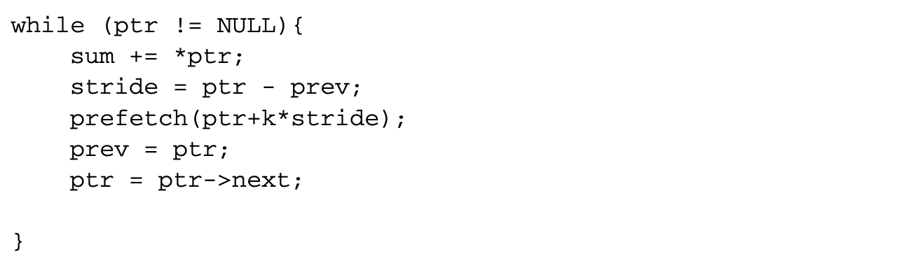The loop contains code to dynamically calculate the stride. Assuming that phases with a particular stride last for a long time, the current observed stride is used to prefetch the pointer that is likely to be accessed $k$ iterations later. Since the overhead of this prefetching is high, it must be employed judiciously after considering factors such as the iteration count of the loop, the average access latency of the load that is prefetched, and the length of the phases with a single stride.

Another type of access that is useful to prefetch is indirect access. In the code fragment 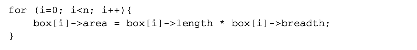the references to the array box can be prefetched. However, the references to area, length, and breadth may cause a large number of cache misses if the pointers stored in the box array do not point to contiguous memory locations. Profile-based prefetching techniques are also not helpful in this case. The solution is to perform indirect prefetching. After applying indirect prefetching, the loop would look like 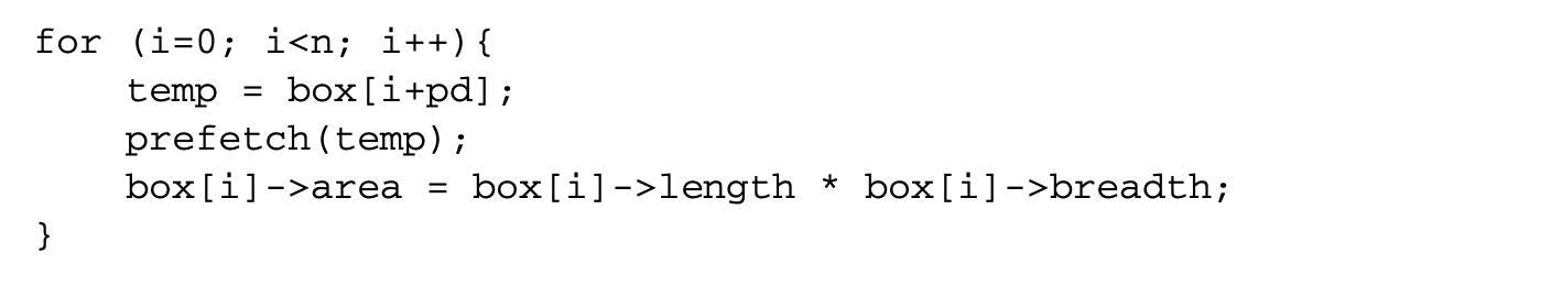The pointer that would be dereferenced pd iterations later is loaded into a temporary variable, and a prefetch is issued for that address. The new loop requires a prefetch to box[i+pd], as otherwise the load to temp could result in stalls that may negate any benefits from indirect prefetching.

5.7 Data Layout Transformations

The techniques discussed so far transform the code accessing the data so as to decrease the memory access latency. An orthogonal approach to reduce memory access latency is to transform the layout of data in memory. For example, if two pieces of data are always accessed close to each other, the spatial locality can be improved by placing those two pieces of data in the same cache line. Data layout transformations are a class of optimization techniques that optimize the layout of data to improve spatial locality. These transformations can be done either within a single aggregate data type or across data objects.

5.7.1 Field Layout

The fields of a record type can be classified as hot or cold depending on their access counts. It is often beneficial to group hot fields together and separate them from cold fields to improve cache utilization. Consider the following record definition: 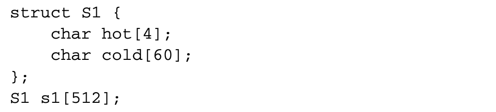Each instance of S1 occupies a single cache line, and the entire array s1 occupies 512 cache lines. The total size of this array is well above the size of L1 cache in most processors, but only 4 bytes of the above record type are used frequently. If the struct consists of only the field hot, then the entire array fits within an L1 cache.

Structure splitting involves separating a set of fields in a record type into a new type and inserting a pointer to this new type in the original record type. Thus, the above struct can be transformed to: 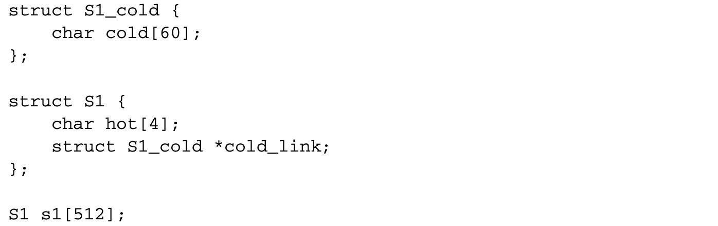After the transformation, the array s1 fits in L1 cache of most processors. While this increases the cost of accessing cold, as it requires one more indirection, this does not hurt much because it is accessed infrequently. However, even this cost can be eliminated for the struct defined above, by transforming S1, as follows: The above transformation is referred to as structure peeling. While peeling is always better than splitting in terms of access costs, it is sometimes difficult to peel a record type. For instance, if a record type has pointers to itself, then peeling becomes difficult.

While merely grouping the hot fields together is often useful, this method suffers from performance penalties when the size of the record is large. As an example, consider the following record definition and some code fragments that use the record: 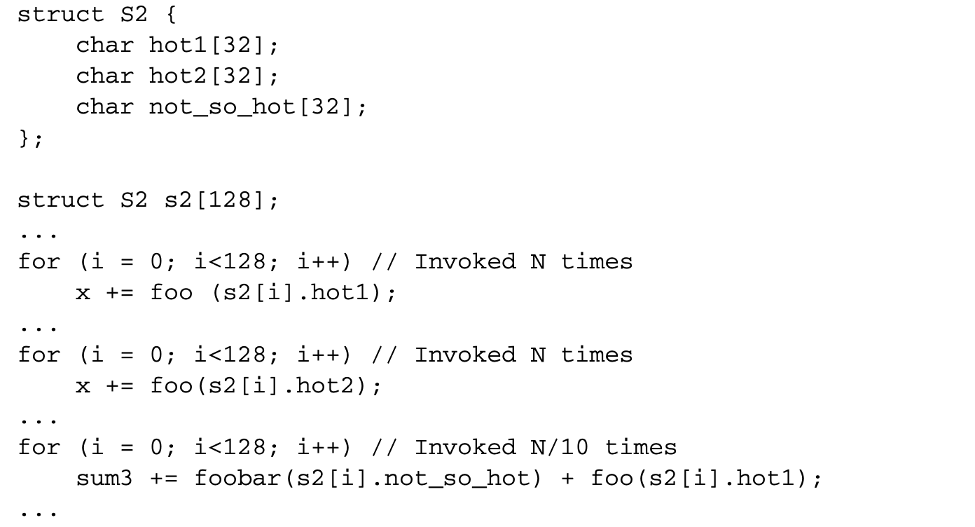The fields hot1 and hot2 are more frequently accessed than not_so_hot, but not_so_hot is always accessed immediately before hot1. Hence placing not_so_hot together with hot1 improves spatial locality and reduces the misses to hot1. This fact is captured by the notion of reference affinity. Two fields have a high reference affinity if they are often accessed close to each other. In the above example, we have considered accesses within the same loop as affine. One could also consider other code granularities such as basic block, procedure, arbitrary loop nest, and so on. Structure splitting, peeling, and re-layout involve the following steps:

1. Determine if it is safe to split a record type. Some examples of the unsafe behaviors include:

• (a) Implicit assumptions on offset of fields. This typically involves taking the address of a field within the record.

• (b) Pointers passed to external routines or library calls. This can be detected using pointer escape analysis.

• (c) Casting from or to the record type under consideration. Casting from type A to type B implicitly assumes a particular relative ordering of the fields in both A and B. If a record type is subjected to any of the above, it is deemed unsafe to transform.

2. Classify the fields of a record type as hot or cold. This involves computing the dynamic access counts of the structure fields. This can be done either using static heuristics or using profiling. Then fields whose access counts are above a certain threshold are labeled as hot and the other fields are labeled as cold.
3. Move the cold fields to a separate record and insert a pointer to this cold record type in the original type.
4. Determine an ordering of the hot fields based on the reference affinity between them. This involves the following steps:
5. Compute reference affinity between all pairs of fields using some heuristic.
6. Group together fields that have high affinity between them.

5.7.2 Data Object Layout

Data object layout attempts to improve the layout of data objects in stack, heap, or global data space. Some of the techniques for field layout are applicable to data object layout as well. For instance, the local variables in a function can be treated as fields of a record, and techniques for field layout can be applied. Similarly, all global variables can likewise be considered as fields of a single record type.

However, additional aspects of the data object layout problem add to its complexity. One such aspect is the issue of cache line conflicts. Two distinct cache lines containing two different data objects may conflict in the cache. If those two data objects are accessed together frequently, a large number of conflict misses may result. Conflicts are usually not an issue in field layout because the size of structures rarely exceeds the size of the cache, while global, stack, and heap data exceed the cache size more often.

Heap layout is usually more challenging because the objects are allocated dynamically. Placing a particular object at some predetermined position relative to some other object in the heap requires the cooperation of the memory allocator. Thus, all heap layout techniques focus on customized memory allocation that uses runtime profiles to guide allocation. The compiler has little role to play in most of these techniques.

A different approach to customized memory allocation, known as pool allocation, has been proposed by Lattner and Adve[14]. Pool allocation identifies the data structure instances used in the program. The allocator then tries to allocate each data structure instance in its own pool. Consider the following code example: 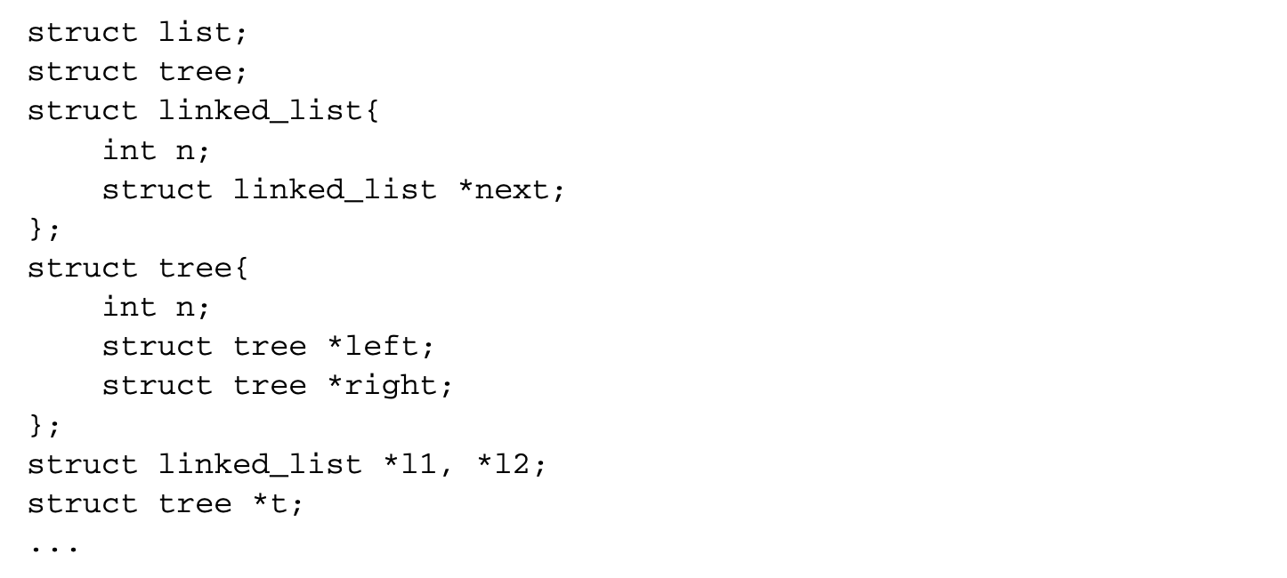Assume that after the necessary dynamic allocations, the pointer l1 points to the head of a linked list, l2 points to the head of a different linked list, and t points to the root of a binary tree. The memory for each of these three distinct data structure instances in the program would be allocated in three distinct pools. Thus, if a single data structure instance is traversed repeatedly without accessing the other instances, the cache will not be polluted by unused data, thereby improving the cache utilization. The drawback to this technique is that it does not profile the code to identify the access patterns and hence may cause severe performance degradation when two instances, such as l1 and l2 above, are concurrently accessed.

5.8 Optimizations for Instruction Caches

Modern processors issue multiple instructions per clock cycle. To efficiently utilize this ability to issue multiple instructions per cycle, the memory system must be able to supply the processor with instructions at a high rate. This requires that the miss rate of instructions in the instruction cache be very low. Several compiler optimizations have been proposed to decrease the access latency for instructions in the instruction cache.

5.8.1 Code Layout in Procedures

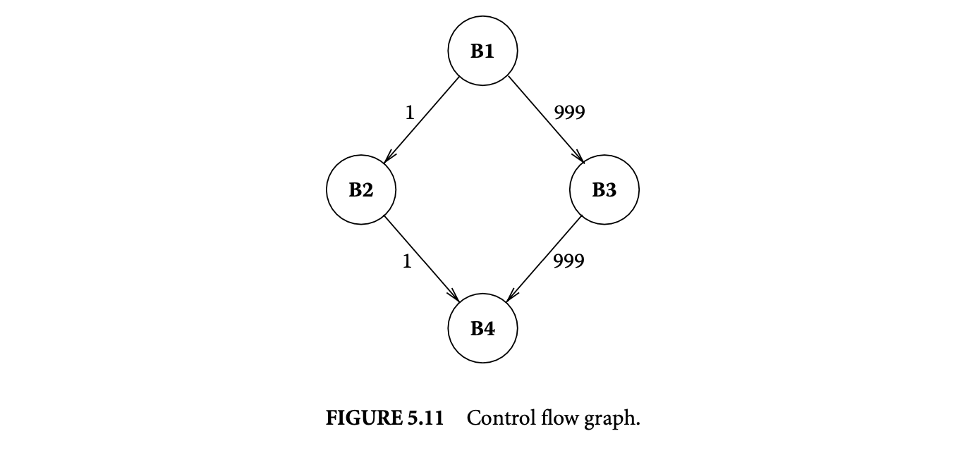
A procedure consists of a set of basic blocks. The mapping from the basic blocks to the virtual address space can have a big impact on the instruction cache performance. Consider the section of control flow graph in Figure 5.11 that corresponds to an if-then-else statement. The numbers on the edges denote the frequency of execution of the edges. Thus, most of the time, the basic block B3 is executed after B1, and B2 is seldom executed. It is not desirable to place B2 after B1, as that could fill the cache line containing B1 with infrequently used code. The code layout algorithms use profile data to guide the mapping of basic blocks to the address space.

Figure 5.12 shows an algorithm proposed by Pettis and Hansen [22] to do profile-guided basic block layout. The algorithm sorts the edges of the control flow graph by the frequency of execution. Initially, every basic block is assumed to be in a chain containing just itself. A chain is simply a straight line path 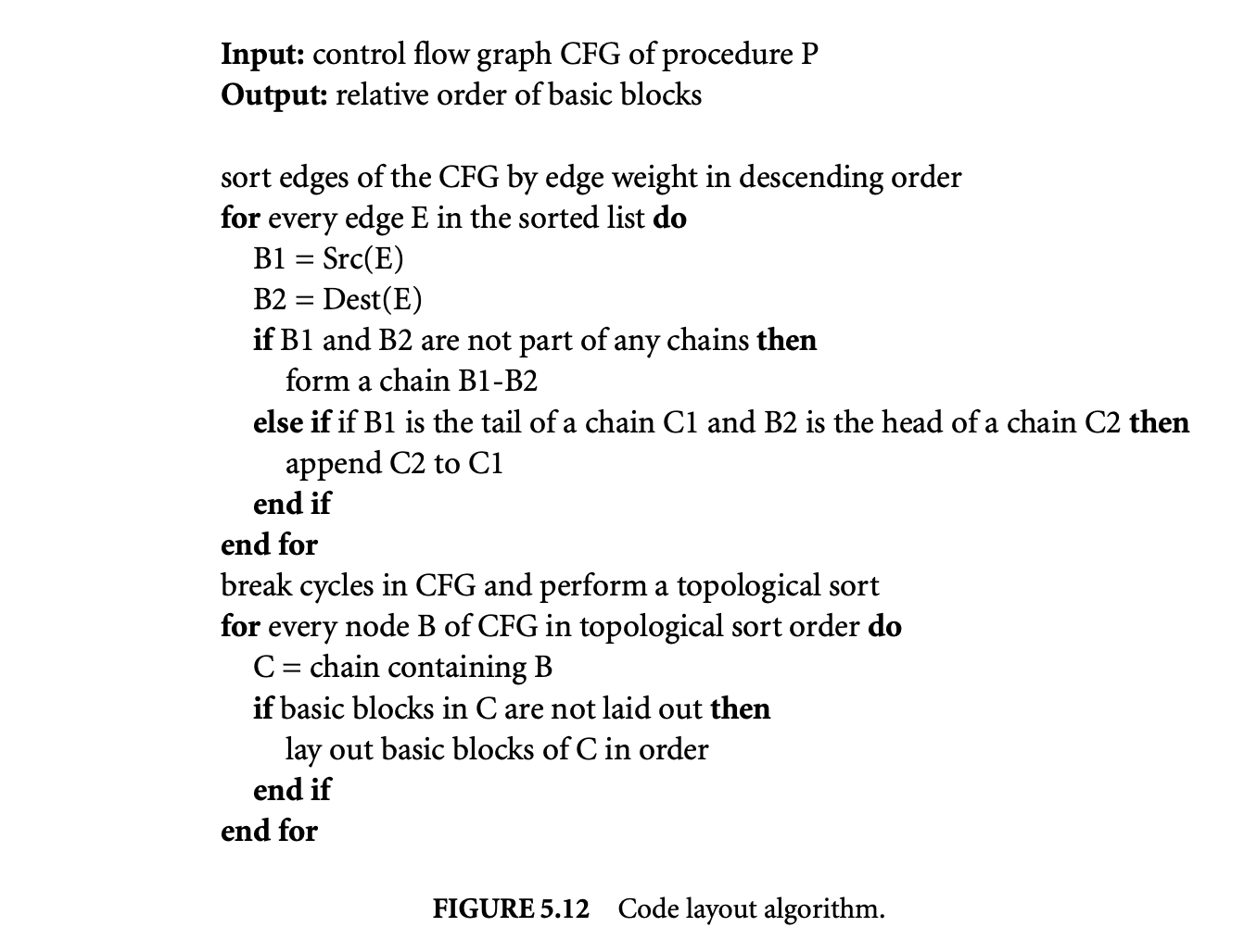in the control flow graph. The algorithm tries to merge the chains into longer chains by looking at each edge, starting from the one with the highest frequency. If the source of the edge is the tail node of a chain and the destination is the head node of a chain, the chains are merged. This process continues until all edges are processed. Then the algorithm does a topological sort of the control flow graph after breaking cycles. The chains corresponding to the nodes in the topological order are laid out consecutively in memory.

5.8.2 Procedure Splitting

While the above algorithm separates hot blocks from cold blocks within a procedure, a poor instruction cache performance still might result. To see this, consider a program with two procedures P1 and P2. Let the hot basic blocks in each procedure occupy one cache line and the cold basic blocks occupy one cache line. If the size of the cache is two cache lines, using the layout produced by the previous algorithm might result in the hot blocks of the two procedures getting mapped to the same cache line, producing a large number of cache misses.

A simple solution to this problem is to place the hot basic blocks of different procedures close to each other. In the above example, this will avoid conflict between the hot basic blocks of the two procedures. Procedure splitting[22] is a technique that splits a procedure into hot and cold sections. Hot sections of all the procedures are placed together, and the cold sections are placed far apart from the hot sections. If the size of the entire program exceeds the cache size, while the hot sections alone fit within the cache, then procedure splitting will result in the cache being occupied by hot code for a large fraction of time. This results in very few misses during the execution of the hot code, resulting in considerable performance improvement.

Procedure splitting simply classifies the basic blocks as hot or cold based on some threshold and moves the cold basic blocks to a distant memory location. For processors that require a special instruction to jump beyond a particular distance, all branches that conditionally jump to a cold basic block are redirected to a stub code, which jumps to the actual cold basic block. Thus, the transitions between hot and cold regions have to be minimal, as they require two control transfer instructions including the costlier special jump instruction.

5.8.3 Cache Line Coloring

Another technique known to improve placement of blocks across procedures is cache line coloring [9]. Cache line coloring attempts to place procedures that call each other in such a way that they do not map to the same set of cache blocks.

Consider the following code fragment:

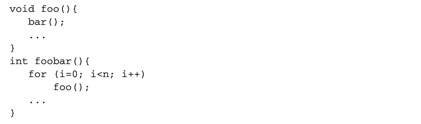
The procedure foolar contains a loop in which foo is called and foo calls bar. The procedures foo and bar must not map to the same cache line, as that will result in a large number of misses. If it is assumed that the size of the hot code blocks in the program exceeds the size of the instruction cache,procedure splitting might still result in the code blocks of foo and bar being mapped to the same set of cache lines.

The input to cache line coloring is the call graph of a program with weighted undirected edges, where the weight on the edge connecting P1 and P2 denotes the number of times P1 calls P2 or vice versa. The nodes are labeled with the number of cache lines required for that procedure. The output of the technique is a mapping between procedures to a set of cache lines. The algorithm tries to minimize the cache line conflicts between nodes that are connected by edges with high edge weights. The edges in the call graph are first sorted by their weights, and each edge is processed in the descending order of weights. If both the nodes connecting an edge have not been assigned to any cache lines, they are assigned nonconflicting cache lines. If one of the nodes is unassigned, the algorithm tries to assign nonconflicting cache lines to the unassigned node without changing the assignment of the other node. If nonconflicting colors cannot be found, it is assigned a cache line close to the other node. If both nodes have already been assigned cache lines, the technique tries to reassign colors to one of them based on several heuristics, which try to minimize the edge weight of edges connected to conflicting nodes.

The main drawback of this technique is that it only considers one level of the call depth. If there is a long call chain, the technique does not attempt to minimize conflicts between nodes in this chain that are adjacent to each other. In addition, the technique assumes that the sizes of procedures are multiples of cache line sizes, which may result in holes between procedures.

5.9 Summary and Future Directions

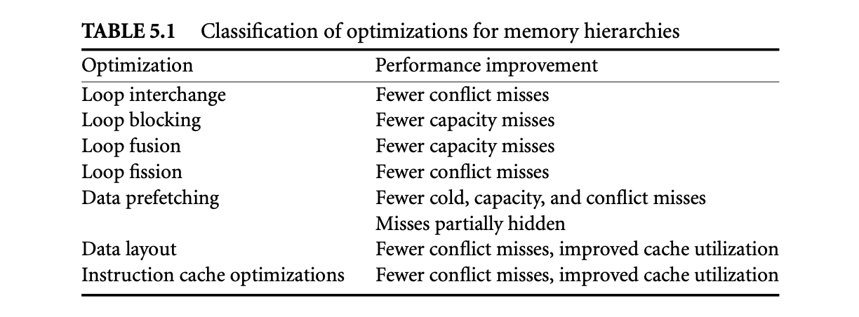
The various optimizations for memory hierarchies described in this chapter are essential components of optimizing compilers targeting modern architectures. While no single technique is a silver bullet for bridging the processor-memory performance gap, many of these optimizations complement each other, and their combination helps a wide range of applications. Table 5.1 summarizes how each of the optimizations achieve improved memory performance.

While these optimizations were motivated by the widening performance gap between the processor and the main memory, the recent trend of stagnant processor clock frequencies may narrow this gap. However, the stagnation of clock frequencies is accompanied by another trend -- the prevalence of chip multiprocessors (CMPs). CMPs pose a new set of challenges to memory performance and increase the importance of compiler-based memory optimizations. Compiler techniques need to focus on multi-threaded applications, as more applications will become multi-threaded to exploit the parallelism offered by CMPs. Compilers also have to efficiently deal with the changes in the memory hierarchy that may have some levels of private caches and some level of caches that are shared among the different cores. The locality in the shared levels of the hierarchy for an application is influenced by applications that are running in the other cores of the CMP.

5.10 References

The work of Abu-Sufah et al. [1] was among the first to look at compiler transformations to improve memory locality. Allen and Kennedy [3] proposed the technique of automatic loop interchange. Loop tiling was proposed by Wolfe [32, 33], who also proposed loop skewing [31]. Several enhancements to tiling including tiling at the register level [11], tiling for imperfectly nested loops [2], and other improvements [12, 27] have been proposed in the literature. Wolf and Lam [29, 30] proposed techniques for combining various unimodular transformations and tiling to improve locality. Detailed discussion of various loop restructuring techniques can be found in textbooks written by Kennedy and Allen [13] and Wolfe [34] and in the dissertations of Porterfield [23] and Wolf [28].

Software prefetching was first proposed by Callahan et al. [5] and Mowry et al. [19, 20, 21]. Machine-specific enhancements to software prefetching have been proposed by Santhanam et al. [26] and Doshi et al. [8]. Luk and Mowry [15] proposed some compiler techniques to prefetch recursive data structures that may not have a strided access pattern. Saavedra-Barrera et al. [25] discuss the combined effects of unimodular transformations, tiling, and software prefetching. Mcintosh [17] discusses various compiler-based prefetching strategies and evaluates them.

Hundt et al. [10] developed an automatic compiler technique for structure layout optimizations. Calder et al. [4] and Chilimbi et al. [6, 7] proposed techniques for data object layout that require some level of programmer intervention or library support. Mcintosh et al. [18] describe an interprocedural optimization technique for placement of global values. Lattner and Adve [14] developed compiler analysis and transformation for pool allocation based on the types of data objects.

McFarling [16] first proposed optimizations targeting instruction cache performances. He gave results on optimal performance under certain assumptions. Pettis and Hansen [22] proposed several profile-guided code positioning techniques including basic block ordering, basic block layout, and procedure splitting. Hashemi et al. [9] proposed the coloring-based approach to minimize cache line conflicts in instruction caches.

References

In IPPS '96: Proceedings of the 10th International Parallel Processing Symposium, 39-45. Washington, DC: IEEE Computer Society.

References

Ken Kennedy and John R. Allen. 2002. Optimizing compilers for modern architectures: A dependence-based approach. San Francisco: Morgan Kaufmann. [19]: Todd C. Mowry. 1995. Tolerating latency through software-controlled data prefetching. PhD thesis, Stanford University, Stanford, CA.